
Overview
The purpose of the control strategy optimization routine is to determine the set of control strategy parameters that meet the user-specified objectives and constraints. It accomplishes this by adjusting the control strategy parameters and reevaluating the performance criteria until all of the specifications have been met. Currently, two forms of this function are active in ADVISOR. The first is Matlab-based and uses one- and two-dimentional multi-level parametric sweeps and some built-in logic to determine the appropriate settings. The second uses VisualDOC optimization software to determine the appropriate settings. Either control strategy optimization routine only provides a single solution to the optimization problem. Therefore, the results should only be used as guide. In both cases, it is recommended but not necessary that the vehicle first be autosized. The control strategy optimization routine will require access to the performance (grade and acceleration) constraint information defined during the autosizing routine. The control strategy optimization routine will confirm that the vehicle continues to meet these constraints while adjusting the design variables. This optimization routine is available for series (includes fuel cell) and parallel hybrid vehicles. The conventional and electric vehicles in ADVISOR don’t have control strategy parameters to be optimized.
Control Strategy Optimization Setup Window
Figure 1 displays the Control Strategy Optimization Setup Window. This interface allows the user to define how the optimization routine will progress and to configure the design variables, objectives, and constraints.

Figure 1: Control Strategy Optimization Setup Window
Optimization Method Selection
Here the user must select the computation engine for the optimization routine. If the “Optimize using VisualDOC” radiobutton is selected ADVISOR will use the VisualDOC optimization software to determine the solution. Otherwise, a custom Matlab-based routine will be used. A limited version of VisualDOC is provided with ADVISOR. If you don’t have a full licensed version of VisualDOC installed on your machine your problem will be limited to 5 design variables.
Cycle/Test Procedure Selection
The user must decide whether to optimize the control strategy parameters for a single drive cycle or for a test procedure. All drive cycles and test procedures available within the Simulation Setup Window are available to the user. Note that optimizing over a test procedure can significantly increase the time required to solve the optimization problem. Also note that a vehicle optimized for a single cycle may not necessarily provide good results on other drive cycles or test procedures.
Design Variable Configuration
In this section, the user must define which design variables should be modified by the optimization routines. Only those design variables selected will by modified, all others will be left unchanged. If using the Matlab-based optimization routine, the cs_lo_soc and the cs_hi_soc variables are unavailable as design variables because these parameters can be more efficiently set within the Matlab-based autosize routine. The user must then define the initial conditions, lower bound, and upper bound for each of the selected design variables. By default the initial conditions are the current parameter values in the Matlab workspace. In addition, if using the Matlab-based routine, the user must specify the number of points in each level of the parametric sweep to be performed. The number of points in the first parametric sweep level defines the course resolution or the number of points to be evaluated between the upper and lower bounds. The number of points in the second parametric sweep level defines the fine resolution or the number of points to be evaluated around the best value of the first parametric sweep. For example, given the following set of inputs,
| upper bound = 1 | number of points in the first sweep = 4 |
| lower bound = 0 | number of points in the second sweep = 3 |
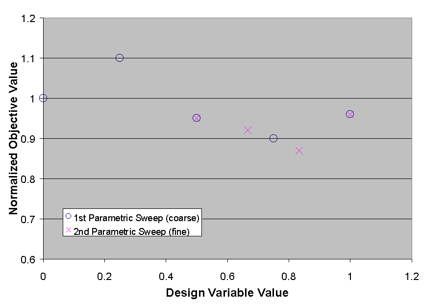
Figure 2: Multi-level Parametric Sweep Graphical Example
During the first parametric sweep the vehicle performance will be evaluated at X = [0 0.25 0.5 0.75 1.0]. Assuming the best results occurred at X = 0.75 then during the second parametric sweep the vehicle performance will be evaluated at X = [0.5 0.666 0.833 1.0]. This example is shown graphically in Figure 2. The optimal setting is determined from the combined data set of both parametric sweeps.
Objective/Constraint Configuration
The user must configure the constraints and objectives to be used in selecting the optimal design variable values. If the “OBJ” radiobutton is selected the parameter will be considered in calculating the normalized objective function. Otherwise, the parameter will be considered as a constraint. To simply ignore a certain parameter select the “CON” radiobutton and enter -1 for the Value. For those parameters specified as objectives the user must specify the weighting factor associated with that parameter. This will determine it’s overall importance in the normalized objective function. Only those parameters specified as active objectives will be included in the objective function calculation. The normalized objective function will be minimized and is calculated as follows,
Equation 1 
Now the optimization routine can be executed by selecting the “RUN” button. You will be offered the opportunity to edit and accept the existing or the default (if autosize routine was not executed) performance constraints that will be enforced. Before the routine will execute an estimate of the time to complete the optimization routine based on the inputs provided is calculated. At this point the user may either continue to execute the routine by selecting “OK” or cancel the routine by selecting “CANCEL”. Selecting cancel will return you to the Control Strategy Optimization Setup Window and allow you to either reconfigure the optimization parameters or exit the setup process. Note that the time estimate is only an estimate and will vary depending on computer processing speeds and the length of the cycle/test procedure selected.
VisualDOC Parameters
This section has been provided for future use. Currently, there are no user-modifiable VisualDOC parameters.
Control Strategy Optimization Plots
During the control optimization routine, various plots are displayed to provide feedback to the user. When using VisualDOC, you will receive two different plots. The first, Figure 3, is displayed during the Design of Experiments stage of the optimization process and shows the value of each design variable relative to its upper and lower bounds. Currently, the routine executes a full second-order Koshal design with interactions (for more information on the Koshal design method please refer to the documentation for VisualDOC). This plot will be updated periodically as the routine executes. The second plot, shown in Figure 4, is displayed during the Optimization Stage of the routine and displays the progress made towards minimizing the normalized objective function at each design iteration. In addition, it shows the value of the variables being optimized. The variable values that have changed from one iteration to the next will be shown in red. The status of the constraint parameters and the contribution to the normalized objective function due to each partial objective are shown. This figure will be updated at each iteration of the optimization process. When the optimization has completed the Plot history buttons will become active and will allow you to view how the design variables were adjusted during the optimization process.

Figure 3: Design Variable Plot Provided During Design of Experiments Stage
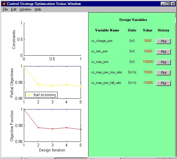
Figure 4: Control Strategy Optimization Status Figure
When using the Matlab-based routine, the plot history function will provide plots similar to those shown below in Figures 5 and 6.
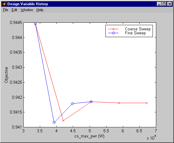
Figure 5: One-Dimensional Parametric Sweep Results Plot
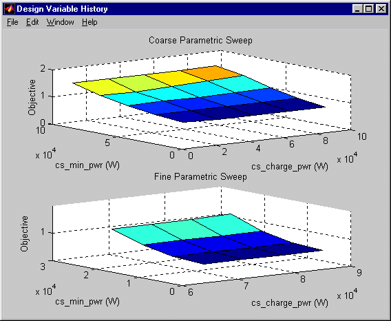
Figure 6: Two-Dimensional Parametric Sweep Results Plot
When using VisualDOC the plot history function will provide plots similar to Figure 7.
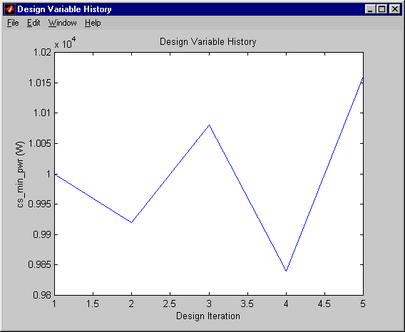
Figure 7: Two-Dimensional Parametric Sweep Results Plot
Control Strategy Optimization Results
After the control strategy optimization routine has completed, all modifications to the vehicle configuration will be detailed in the Matlab command window and all values will be updated in the ADVISOR edited variable list as shown in Figure 9. At this point, it is recommended that you return to the Vehicle Setup Window and save your vehicle so that the results will be available for future analysis.
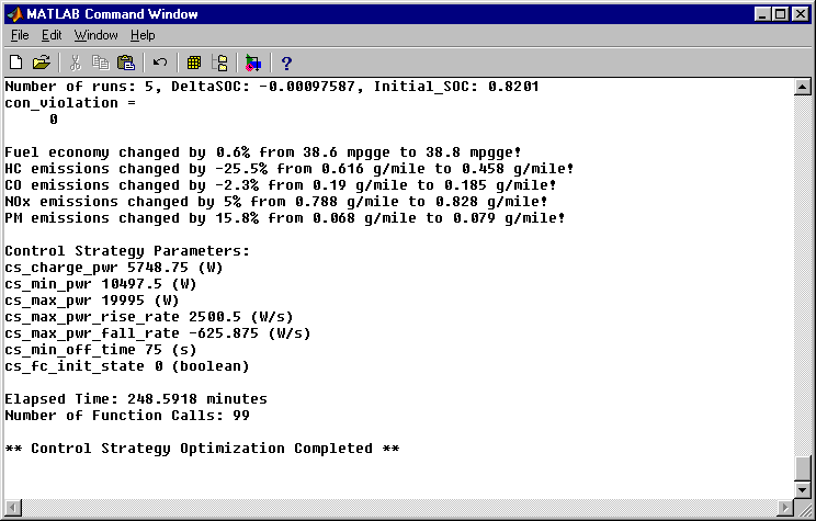
Figure 9: Matlab Command Window Summary Messages
Control Strategy Optimization using Matlab-based Routine
The Matlab-based control strategy optimization routine uses one- and two-dimensional multi-level parametric sweeps to determine the optimal control strategy parameter settings based on the user-specified objectives and constraints. This routine also uses built-in logic and knowledge of the optimization problem to find a solution relatively quickly. It does not ensure that this is the global optimum and it does not consider the interactions between all design variables.
First the performance of the current vehicle is evaluated and stored for use in calculating the objective function. Then the active design variables are set to values that will not restrict the performance of the vehicle. These initial parameter values are listed in Table 1 below.
Table 1: Initial Parameter Settings
|
Variable Name |
Value |
|
Series |
|
|
cs_charge_pwr |
0 |
|
cs_min_pwr |
0 |
|
cs_max_pwr |
Inf |
|
cs_max_pwr_rise_rate |
Inf |
|
cs_max_pwr_fall_rate |
-inf |
|
cs_min_off_time |
0 |
|
cs_fc_init_state |
0 |
|
Parallel |
|
|
cs_charge_trq |
0 |
|
cs_min_trq_frac |
0 |
|
cs_off_trq_frac |
0 |
|
cs_electric_launch_spd |
0 |
The routine then explores the user-defined range of each active design variable and sets the variable to its optimal setting. The order in which the variables are evaluated and assigned new values follows the order of the variable listings in Table 1 for the specific vehicle-type. This order has been determined based on relative impact (from most to least effective) of each parameter on vehicle performance and is the same as the order in which the variables are displayed in the Control Strategy Optimization Setup Window.
In addition, for both series and parallel vehicles, there are linked variables that must be evaluated together if both variables are active design variables. For series vehicles, cs_charge_pwr and cs_min_pwr are linked variables. For parallel vehicles, cs_charge_trq and cs_min_trq_frac are linked variables. Two-dimensional multi-level parametric sweeps are used for these variables. All other variables are evaluated independently using one-dimensional multi-level parametric sweeps.
Once the routine has set all parameters to the best values it compares the resulting vehicle performance to the initial vehicle performance (prior to any overrides) to ensure that the objective function has improved. If the objective function has not improved the initial vehicle settings are restored. If it has improved, the summary information is provided in the Matlab command window.
VisualDOC is a gradient based optimization software package to be used with various other codes and software packages. The control strategy optimization routine using VisualDOC proceeds as follows,
To use the VisualDOC-based routine, a licensed version of VisualDOC 1.2 must be installed on the computer. To obtain a full licensed version of VisualDOC 1.2, contact VanderPlatts R&D at http:\\www.vrand.com. A limited demonstration version of VisualDOC is inclued with ADVISOR and this allows the user to execute optimization problems with 5 or less design variables.
The VisualDOC-based routine does consider interactions between design variables but still does not ensure that the solution is a global optimum.
When using the VisualDOC-based routine it is possible to perform multiple optimization runs using the same DOE data set. During the first execution of the control strategy optimization routine a DOE data set will be created. The response surface approximations routine uses this data set to determine the optimum settings based on the user-defined objectives and constraints. On completion of the optimization, the user may decide that he/she would like to optimize for a different set of objectives and constraints. When the Optimize Control Strategy button is selected, the user will be prompted to use the existing DOE or generate a new DOE data set. If you use the existing data set you will only be allowed to change the objective and constraint settings and edit the conditions of the previously active design variables. All simulation parameters must be left unchanged for the DOE data set to be valid. If you decide to generate a new data set you will be able to modify any of the input parameters, but the routine will take significantly more time to complete.
Last Revised: 10/27/99:tm